Example: Variational Auto-Encoder
This section covers Section 3 of the paper: a concrete implementation using neural networks.
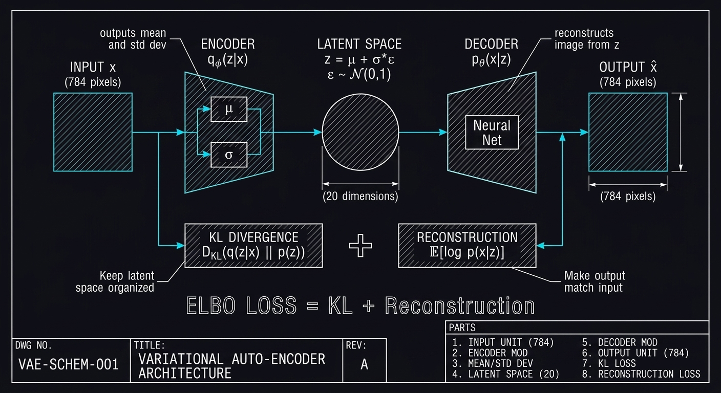 The complete VAE architecture showing the encoder (left) producing mean μ and standard deviation σ, the latent space sampling (center), and the decoder (right) reconstructing the output. The bottom shows the two loss components: KL Divergence and Reconstruction.
The Setup
The paper presents a specific instantiation of the AEVB framework:
- Encoder: Neural network for $q_\phi(\mathbf{z}|\mathbf{x})$
- Decoder: Neural network for $p_\theta(\mathbf{x}|\mathbf{z})$
- Both trained jointly with the AEVB algorithm
Prior Distribution
The prior over latent variables is chosen to be the centered isotropic multivariate Gaussian:
$$p_\theta(\mathbf{z}) = \mathcal{N}(\mathbf{z}; \mathbf{0}, \mathbf{I})$$
Note: This prior has no learnable parameters. This is a design choice, not a limitation.
Decoder (Generative Model)
The decoder $p_\theta(\mathbf{x}|\mathbf{z})$ can be either:
For Real-Valued Data: Gaussian Decoder
$$p_\theta(\mathbf{x}|\mathbf{z}) = \mathcal{N}(\mathbf{x}; \boldsymbol{\mu}\theta(\mathbf{z}), \boldsymbol{\sigma}^2\theta(\mathbf{z})\mathbf{I})$$
Where $\boldsymbol{\mu}\theta(\mathbf{z})$ and $\boldsymbol{\sigma}^2\theta(\mathbf{z})$ are outputs of an MLP.
For Binary Data: Bernoulli Decoder
$$p_\theta(\mathbf{x}|\mathbf{z}) = \prod_{i=1}^{D} \text{Bernoulli}(x_i; y_i)$$
Where $\mathbf{y} = f_\sigma(\mathbf{W}_2 \tanh(\mathbf{W}_1 \mathbf{z} + \mathbf{b}_1) + \mathbf{b}_2)$
And $f_\sigma(\cdot)$ is the sigmoid function.
The log-likelihood for Bernoulli:
$$\log p(\mathbf{x}|\mathbf{z}) = \sum_{i=1}^{D} x_i \log y_i + (1 - x_i) \log(1 - y_i)$$
Encoder (Recognition Model)
The true posterior $p_\theta(\mathbf{z}|\mathbf{x})$ is intractable. The paper assumes it’s approximately Gaussian with approximately diagonal covariance.
Equation (9): Gaussian Encoder
$$\log q_\phi(\mathbf{z}|\mathbf{x}^{(i)}) = \log \mathcal{N}(\mathbf{z}; \boldsymbol{\mu}^{(i)}, \boldsymbol{\sigma}^{2(i)}\mathbf{I})$$
Where $\boldsymbol{\mu}^{(i)}$ and $\boldsymbol{\sigma}^{(i)}$ are outputs of the encoding MLP:
- They are nonlinear functions of datapoint $\mathbf{x}^{(i)}$
- They depend on variational parameters $\phi$
Encoder MLP Architecture
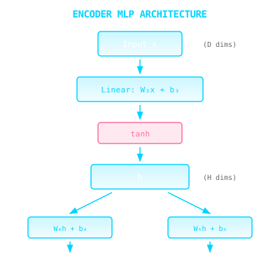 The encoder network maps input x through a hidden layer to produce both the mean μ and log-variance log σ² of the approximate posterior.
Parameters: $\phi = {\mathbf{W}_3, \mathbf{W}_4, \mathbf{W}_5, \mathbf{b}_3, \mathbf{b}_4, \mathbf{b}_5}$
Why log σ²? The network outputs $\log \boldsymbol{\sigma}^2$ instead of $\boldsymbol{\sigma}$ directly because:
- $\boldsymbol{\sigma}$ must be positive, but network outputs can be any real number
- $\log \boldsymbol{\sigma}^2$ can be any real number
- $\boldsymbol{\sigma} = \exp(\frac{1}{2} \log \boldsymbol{\sigma}^2)$ is always positive
Sampling via Reparameterization
As explained in Section 2.4, we sample from the posterior using:
$$\mathbf{z}^{(i,l)} = g_\phi(\mathbf{x}^{(i)}, \boldsymbol{\epsilon}^{(l)}) = \boldsymbol{\mu}^{(i)} + \boldsymbol{\sigma}^{(i)} \odot \boldsymbol{\epsilon}^{(l)}$$
Where $\boldsymbol{\epsilon}^{(l)} \sim \mathcal{N}(\mathbf{0}, \mathbf{I})$ and $\odot$ is element-wise product.
The Final Estimator — Equation (10)
Since both $p_\theta(\mathbf{z})$ (prior) and $q_\phi(\mathbf{z}|\mathbf{x})$ (encoder) are Gaussian, we can use estimator B with analytical KL divergence:
$$\mathcal{L}(\theta, \phi; \mathbf{x}^{(i)}) \simeq \frac{1}{2} \sum_{j=1}^{J} \left(1 + \log((\sigma_j^{(i)})^2) - (\mu_j^{(i)})^2 - (\sigma_j^{(i)})^2\right) + \frac{1}{L} \sum_{l=1}^{L} \log p_\theta(\mathbf{x}^{(i)}|\mathbf{z}^{(i,l)})$$
Where:
- $J$ is the dimensionality of the latent space
- $\mathbf{z}^{(i,l)} = \boldsymbol{\mu}^{(i)} + \boldsymbol{\sigma}^{(i)} \odot \boldsymbol{\epsilon}^{(l)}$
- $\boldsymbol{\epsilon}^{(l)} \sim \mathcal{N}(\mathbf{0}, \mathbf{I})$
Breaking Down Equation (10)
| Term | Expression | Meaning |
|---|---|---|
| KL term | $\frac{1}{2} \sum_{j=1}^{J} (1 + \log \sigma_j^2 - \mu_j^2 - \sigma_j^2)$ | Analytical KL divergence (no sampling!) |
| Reconstruction | $\frac{1}{L} \sum_{l=1}^{L} \log p_\theta(\mathbf{x}^{(i)} | \mathbf{z}^{(i,l)})$ |
The Reconstruction Term in Practice
For Bernoulli Decoder (Binary Data like MNIST):
$$\log p_\theta(\mathbf{x}|\mathbf{z}) = \sum_{i=1}^{D} x_i \log y_i + (1 - x_i) \log(1 - y_i)$$
This is the binary cross-entropy between input $\mathbf{x}$ and decoder output $\mathbf{y}$.
For Gaussian Decoder (Continuous Data):
$$\log p_\theta(\mathbf{x}|\mathbf{z}) = -\frac{D}{2} \log(2\pi) - \frac{1}{2} \sum_{i=1}^{D} \left(\log \sigma_i^2 + \frac{(x_i - \mu_i)^2}{\sigma_i^2}\right)$$
Often simplified (with fixed $\sigma = 1$) to:
$$\log p_\theta(\mathbf{x}|\mathbf{z}) \propto -\frac{1}{2} |\mathbf{x} - \boldsymbol{\mu}_\theta(\mathbf{z})|^2$$
This is the mean squared error (up to constants).
Complete VAE Architecture Summary
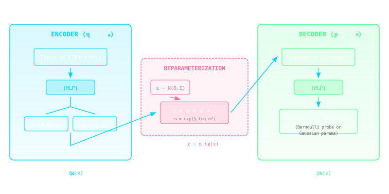 The full VAE architecture showing the encoder producing distribution parameters, the reparameterization trick sampling z, and the decoder reconstructing the output.
PyTorch-Style Pseudocode
class VAE(nn.Module):
    def __init__(self, input_dim, hidden_dim, latent_dim):
        # Encoder
        self.encoder_fc = nn.Linear(input_dim, hidden_dim)
        self.fc_mu = nn.Linear(hidden_dim, latent_dim)
        self.fc_logvar = nn.Linear(hidden_dim, latent_dim)

        # Decoder
        self.decoder_fc = nn.Linear(latent_dim, hidden_dim)
        self.decoder_out = nn.Linear(hidden_dim, input_dim)

    def encode(self, x):
        h = torch.tanh(self.encoder_fc(x))
        mu = self.fc_mu(h)
        logvar = self.fc_logvar(h)
        return mu, logvar

    def reparameterize(self, mu, logvar):
        std = torch.exp(0.5 * logvar)  # σ = exp(½ log σ²)
        eps = torch.randn_like(std)     # ε ~ N(0, I)
        return mu + std * eps           # z = μ + σ ⊙ ε

    def decode(self, z):
        h = torch.tanh(self.decoder_fc(z))
        return torch.sigmoid(self.decoder_out(h))

    def forward(self, x):
        mu, logvar = self.encode(x)
        z = self.reparameterize(mu, logvar)
        x_recon = self.decode(z)
        return x_recon, mu, logvar

def loss_function(x_recon, x, mu, logvar):
    # Reconstruction loss (binary cross-entropy)
    BCE = F.binary_cross_entropy(x_recon, x, reduction='sum')

    # KL divergence (analytical, Equation 10)
    # -0.5 * sum(1 + log(σ²) - μ² - σ²)
    KLD = -0.5 * torch.sum(1 + logvar - mu.pow(2) - logvar.exp())

    return BCE + KLD
Key Design Choices
| Choice | Paper’s Decision | Rationale |
|---|---|---|
| Prior | $\mathcal{N}(\mathbf{0}, \mathbf{I})$ | Simple, no parameters to learn |
| Encoder output | $\boldsymbol{\mu}, \log \boldsymbol{\sigma}^2$ | Ensures positive variance |
| Covariance structure | Diagonal | Tractable KL, efficient computation |
| Activation | tanh | Common choice for hidden layers |
| Output (binary) | Sigmoid | Bernoulli probabilities in [0,1] |